#!pip install rasterioIntroduction to Rasterio
A short tutorial using Rasterio in Python
Rasterio
is a Python library that simplifies the reading, writing, and processing of geospatial raster data. It provides a user-friendly interface built on top of GDAL, making it easier to work with raster datasets, handle metadata, and perform spatial operations efficiently in Python. (description from ChatGPT4o)
1 Install/Load Rasterio
I will show you how to Install Rasterio, and then load it to use in python.
Install Rasterio using pip.
This line of code below is commented out because if you have loaded the environment from the environment file (ATUR-WIKI.yml) they should already be installed. If you have not loaded the environment or want to create your own uncomment the line below and run it
2 Load rasterio
import rasterio
from rasterio.plot import show
3 Open a Raster dataset from a URL using Rasterio
# URL of the .tif file. URL to 1/3 arcsecond (10m) National Elevation Dataset DEM
tif_url = 'https://prd-tnm.s3.amazonaws.com/StagedProducts/Elevation/1/TIFF/historical/n35w111/USGS_1_n35w111_20240402.tif'

# Open the raster
dataset = rasterio.open(tif_url)
3.1 Display basic metadata
print(f"CRS: {dataset.crs}")  # Coordinate Reference System
print(f"Bounds: {dataset.bounds}")  # Spatial extent of the raster
print(f"Width: {dataset.width}, Height: {dataset.height}")  # Dimensions
print(f"Number of bands: {dataset.count}")
CRS: EPSG:4269
Bounds: BoundingBox(left=-111.00166666698249, bottom=33.998333332817936, right=-109.99833333361585, top=35.001666667083896)
Width: 3612, Height: 3612
Number of bands: 14 Reading the Raster Data as a NumPyArray
# read the first band (assuming a single-band raster)
band1 = dataset.read(1)

# Display the shape and basic statistics
print(f"Band 1 shape: {band1.shape}")
print(f"Min: {band1.min()}, Max: {band1.max()}")
Band 1 shape: (3612, 3612)
Min: 1324.57958984375, Max: 2410.2331542968755 Visualizing the Raster using Matplotlib
Rasterio integrates well with matplotlib for visualizing raster data
If matplotlib is not installed (i.e. you get an error when you run the next line) use !pip install matplotlib
# import the matplotlib library.
import matplotlib.pyplot as plt

# Plot the raster data using matplotlib and the  viridis colormap

plt.figure(figsize=(10, 8))
plt.imshow(band1, cmap='viridis')
plt.colorbar(label='Elevation (meters)')
plt.title('Elevation Data Visualization')
plt.xlabel('X Pixels')
plt.ylabel('Y Pixels')
plt.show()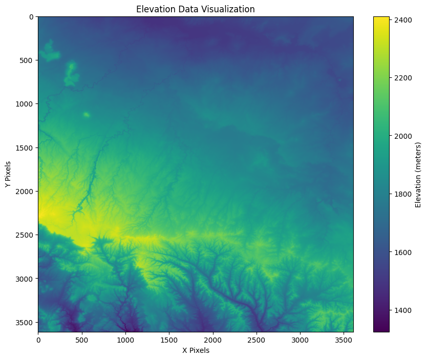
6 Accessing Raster Metadata
Rasterio provides easy access to import metadata like the transform, resolution, and affine transformations
# Get the affine transform (maps pixel coordinates to geographic coordinates)
print(f"Affine transform: {dataset.transform}")

# Get the resolution (pixel size)
print(f"Pixel resolution: {dataset.res}")
Affine transform: | 0.00, 0.00,-111.00|
| 0.00,-0.00, 35.00|
| 0.00, 0.00, 1.00|
Pixel resolution: (0.000277777777786999, 0.00027777777803598015)7 Extracting Specific Pixel Values
You can extract specific pixel values or geographic locations easily with Rasterio
# Example: Extract the value at pixel (500, 500)
row, col = 500, 500
value = band1[row, col]
print(f"Value at pixel (500, 500): {value}")

# Convert pixel coordinates to geographic coordinates
geo_coords = dataset.xy(row, col)
print(f"Geographic coordinates: {geo_coords}")
Value at pixel (500, 500): 1695.1978759765625
Geographic coordinates: (np.float64(-110.8626388892001), np.float64(34.862638889176885))8 Writing Data to New COG
Key Options:
driver='COG': This specifies that the output file should be in Cloud Optimized GeoTIFF format.BLOCKSIZE=512: This sets the internal tile size (512x512 pixels).compress='LZW': This applies LZW compression to reduce the file size.overview_resampling='nearest': This generates overviews using nearest-neighbor resampling, which speeds up access at different zoom levels.
# Define the output path for the COG
output_cog_path = 'output_cog.tif'

# Write the data to a new COG file
with rasterio.open(
    output_cog_path, 'w',
    driver='COG',  # Set driver to COG
    height=band1.shape[0],
    width=band1.shape[1],
    count=1,  # Number of bands
    dtype=band1.dtype,
    crs=dataset.crs,
    transform=dataset.transform,
    BLOCKSIZE=512,  # Set block size for tiling
    compress='LZW',  # Compression to reduce file size
    overview_resampling='nearest'  # Generate overviews for faster access at multiple zoom levels
) as dst:
    dst.write(band1, 1)  # Write the data to the first band

print(f"COG created and saved at: {output_cog_path}")
COG created and saved at: output_cog.tif9 close the dataset
lets free up the RAM by closing this dataset now that we are done.
dataset.close()